Real-time artifact correction comparison#

This example generates a realistic EEG recording with simulate_nf_session(), injects it into a local LSL stream with PlayerLSL, and compares four artifact handling approaches applied in real time as data arrives window-by-window:

AdaptiveLMSFilter — reference-based adaptive filter.
ASRDenoiser — baseline-calibrated subspace rejection.
GEDAIDenoiser — band-selective eigendecomposition.
ORICA — online independent component analysis.

simulate_nf_session() produces 64-channel biosemi64 EEG with realistic 1/f background, alpha oscillations, eye blinks, muscle bursts, slow drift, and an NF-state marker — no MRI data required.

Generate simulated NF session data#

simulate_nf_session() returns a RawArray and a boolean NF-state mask. We use it as our ground truth and stream it via PlayerLSL.

import os
import tempfile
import time

import numpy as np
import matplotlib.pyplot as plt
import mne
from scipy.signal import welch

from mne_rt.tools import (
    simulate_nf_session,
    AdaptiveLMSFilter, ASRDenoiser, GEDAIDenoiser, ORICA,
)
from mne_lsl.player import PlayerLSL
from mne_lsl.stream import StreamLSL

mne.set_log_level("WARNING")

DURATION = 60.0          # seconds
SFREQ    = 256.0
N_CAL    = int(5 * SFREQ)  # first 5 s: clean calibration window

raw_sim, nf_state = simulate_nf_session(
    duration=DURATION,
    sfreq=SFREQ,
    n_channels=64,
    n_blinks=20,
    alpha_amplitude=15e-6,
    background_amplitude=5e-6,
    muscle_rate=0.06,
    alpha_reactivity=True,
    rng_seed=42,
    verbose=False,
)

info     = raw_sim.info
EEG_NAMES = raw_sim.ch_names
N_EEG     = len(EEG_NAMES)
t         = raw_sim.times
print(f"Simulated EEG: {N_EEG} channels  |  {DURATION:.0f} s  |  {SFREQ:.0f} Hz")
print(f"NF state active: {nf_state.mean()*100:.0f} % of samples")

Simulated EEG: 64 channels  |  60 s  |  256 Hz
NF state active: 50 % of samples

Fit calibration-dependent denoisers#

ASR and GEDAI require a short clean calibration segment before the live session. We use the first 5 s of the simulation (before any blinks or muscle bursts are injected at full rate).

data_sim = raw_sim.get_data()

# Build a synthetic EOG reference from frontal channels (Fp1/Fp2)
fp1_idx = EEG_NAMES.index("Fp1") if "Fp1" in EEG_NAMES else 0
fp2_idx = EEG_NAMES.index("Fp2") if "Fp2" in EEG_NAMES else 1
eog_ref  = 0.5 * (data_sim[fp1_idx] + data_sim[fp2_idx])

# Extend data matrix with EOG reference row so LMS has a reference channel
data_with_ref = np.vstack([data_sim, eog_ref[np.newaxis]])
N_WITH_REF    = data_with_ref.shape[0]

cal_data   = data_sim[:, :N_CAL]
chunk_size = int(SFREQ)

asr = ASRDenoiser(cutoff=5.0)
asr.fit(cal_data, sfreq=SFREQ, window_len=1.0)

gedai = GEDAIDenoiser(n_channels=N_EEG)
gedai.fit_from_raw(cal_data, sfreq=SFREQ, band=(8.0, 30.0))
n_noise    = max(2, int(0.20 * N_EEG))
art_idx_g  = gedai.find_noise_components(n_noise=n_noise)

print(f"ASR fitted  |  GEDAI fitted ({len(art_idx_g)} artifact components)")

ASR fitted  |  GEDAI fitted (12 artifact components)

Stream via PlayerLSL and apply corrections in real time#

We save the simulation to a FIF file, start a PlayerLSL, connect with StreamLSL, and process every 1-second chunk through each corrector.

STREAM_NAME = "ANT_ArtComp_demo"
SOURCE_ID   = STREAM_NAME

with tempfile.NamedTemporaryFile(suffix="_raw.fif", delete=False) as _f:
    _tmp_path = _f.name
raw_sim.save(_tmp_path, overwrite=True, verbose=False)

player = PlayerLSL(_tmp_path, chunk_size=chunk_size, name=STREAM_NAME,
                   source_id=SOURCE_ID, n_repeat=1)
player.start()
time.sleep(2.0)

stream = StreamLSL(bufsize=4.0, source_id=SOURCE_ID)
stream.connect(acquisition_delay=0.005, timeout=15.0)
print(f"Streaming: {STREAM_NAME}  |  sfreq={stream.info['sfreq']:.0f} Hz  |  "
      f"n_ch={stream.info['nchan']}")

lms      = AdaptiveLMSFilter(ref_ch_idx=N_EEG, n_taps=8, mu=0.005)
orica    = ORICA(n_channels=N_EEG, learning_rate=0.005, block_size=chunk_size)

data_lms   = np.zeros_like(data_sim)
data_asr   = np.zeros_like(data_sim)
data_gedai = np.zeros_like(data_sim)
data_orica = np.zeros_like(data_sim)

n_chunks   = int(DURATION) // 1
t_deadline = time.perf_counter() + DURATION + 15.0
k = 0

while k < n_chunks and time.perf_counter() < t_deadline:
    if stream.n_new_samples < chunk_size:
        time.sleep(0.005)
        continue

    chunk, _ = stream.get_data(winsize=1.0)        # (n_ch, chunk_size)
    sl = slice(k * chunk_size, (k + 1) * chunk_size)

    # Extend chunk with EOG ref for LMS
    eog_chunk = 0.5 * (chunk[fp1_idx] + chunk[fp2_idx])
    chunk_with_ref = np.vstack([chunk, eog_chunk[np.newaxis]])

    # LMS
    lms_out = lms.transform(chunk_with_ref)
    data_lms[:, sl] = lms_out[:N_EEG]

    # ASR
    data_asr[:, sl] = asr.transform(chunk)

    # GEDAI
    data_gedai[:, sl] = gedai.denoise(chunk, art_idx_g)

    # ORICA — update online
    src = orica.transform(chunk)
    # Re-project with estimated artifact components zeroed (use blink correlation)
    corr_eog = np.array([abs(np.corrcoef(src[i], eog_chunk)[0, 1]) for i in range(N_EEG)])
    n_art    = max(1, int(0.10 * N_EEG))
    art_comps = list(np.argsort(corr_eog)[::-1][:n_art])
    data_orica[:, sl] = orica.denoise(chunk, art_comps)

    k += 1

stream.disconnect()
try:
    player.stop()
except RuntimeError:
    pass
os.unlink(_tmp_path)

print(f"Processed {k} windows via LSL streaming")

Streaming: ANT_ArtComp_demo  |  sfreq=256 Hz  |  n_ch=64
/opt/homebrew/Cellar/python@3.14/3.14.3_1/Frameworks/Python.framework/Versions/3.14/lib/python3.14/concurrent/futures/thread.py:73: RuntimeWarning: ANT_ArtComp_demo: End of file reached with an empty chunk. This should not happen with a chunk_size different from 1.
  return fn(*args, **kwargs)
Processed 57 windows via LSL streaming

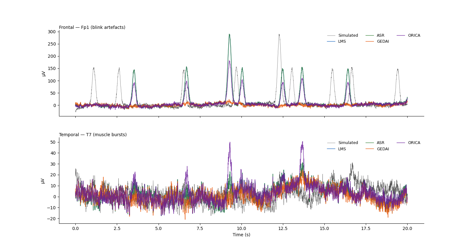
Figure 1 — Time-series comparison#

COLORS = {
    "Simulated": "#555555", "LMS": "#1565C0",
    "ASR": "#2E7D32", "GEDAI": "#E65100", "ORICA": "#6A1B9A",
}

t20  = t[t <= 20.0]
s20  = slice(0, len(t20))

frontal_ch = "Fp1" if "Fp1" in EEG_NAMES else EEG_NAMES[0]
temporal_ch = "T7" if "T7" in EEG_NAMES else EEG_NAMES[1]
ch_rows = [
    (EEG_NAMES.index(frontal_ch),  f"Frontal — {frontal_ch} (blink artefacts)"),
    (EEG_NAMES.index(temporal_ch), f"Temporal — {temporal_ch} (muscle bursts)"),
]

fig1, axes = plt.subplots(2, 1, figsize=(15, 8), sharex=True,
                           gridspec_kw={"hspace": 0.25})

for ax, (ch, title) in zip(axes, ch_rows):
    ax.plot(t20, data_sim[ch, s20] * 1e6,
            color=COLORS["Simulated"], lw=0.5, label="Simulated")
    for mname, mdata in [("LMS", data_lms), ("ASR", data_asr),
                         ("GEDAI", data_gedai), ("ORICA", data_orica)]:
        ax.plot(t20, mdata[ch, s20] * 1e6, color=COLORS[mname],
                lw=1.2, alpha=0.8, label=mname)
    ax.set_ylabel("µV", fontsize=10)
    ax.set_title(title, fontsize=10, loc="left", pad=3)
    ax.legend(fontsize=9, frameon=False, loc="upper right", ncol=3)
    ax.spines[["top", "right"]].set_visible(False)

axes[-1].set_xlabel("Time (s)", fontsize=10)
fig1.tight_layout()

Frontal — Fp1 (blink artefacts), Temporal — T7 (muscle bursts)

/Users/payamsadeghishabestari/ANT/examples/ex_artifact_comparison.py:211: UserWarning: This figure includes Axes that are not compatible with tight_layout, so results might be incorrect.
  fig1.tight_layout()

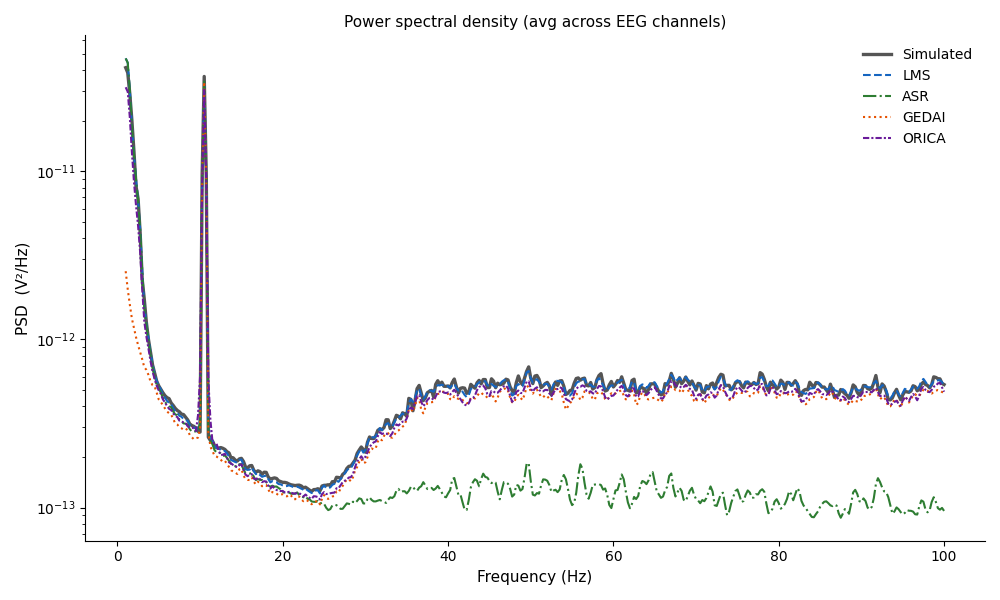
Figure 2 — PSD comparison#

fig2, ax_psd = plt.subplots(1, 1, figsize=(10, 6))
psd_kw = dict(fs=SFREQ, nperseg=int(4 * SFREQ), noverlap=int(2 * SFREQ))
psd_sets = [
    ("Simulated", data_sim,   COLORS["Simulated"], dict(lw=2.4, ls="-")),
    ("LMS",       data_lms,   COLORS["LMS"],       dict(lw=1.5, ls="--")),
    ("ASR",       data_asr,   COLORS["ASR"],       dict(lw=1.5, ls="-.")),
    ("GEDAI",     data_gedai, COLORS["GEDAI"],     dict(lw=1.5, ls=":")),
    ("ORICA",     data_orica, COLORS["ORICA"],     dict(lw=1.5, ls=(0, (3, 1, 1, 1)))),
]

for label, dat, col, kw in psd_sets:
    psds  = [welch(dat[i], **psd_kw)[1] for i in range(dat.shape[0])]
    f_arr = welch(dat[0], **psd_kw)[0]
    mask  = (f_arr >= 1.0) & (f_arr <= 100.0)
    ax_psd.semilogy(f_arr[mask], np.mean(psds, axis=0)[mask], color=col, label=label, **kw)

ax_psd.set_xlabel("Frequency (Hz)", fontsize=11)
ax_psd.set_ylabel("PSD  (V²/Hz)", fontsize=11)
ax_psd.set_title("Power spectral density (avg across EEG channels)", fontsize=11)
ax_psd.legend(fontsize=10, frameon=False)
ax_psd.spines[["top", "right"]].set_visible(False)

fig2.tight_layout()

Power spectral density (avg across EEG channels)

Total running time of the script: (1 minutes 19.265 seconds)

Gallery generated by Sphinx-Gallery