Complete closed-loop NF session

Full end-to-end pipeline with ANT:

1. Simulate a 64-channel EEG recording with a strong, rhythmic alpha modulation pattern — 10 s alpha-ON bursts alternating with 10 s silence.

2. Stream it through a mock LSL player.

3. Record a resting-state baseline and compute the noise covariance.

4. Run a 100-second closed-loop NF session extracting four modalities in parallel.

5. Save the NF data (JSON + BIDS-compatible TSV) and generate an HTML report.

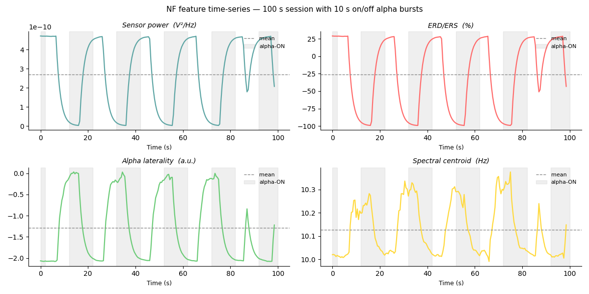
6. Inspect the feature time-series — the 10 s on / 10 s off alpha rhythm is clearly visible as modulation in every NF feature.

The three interactive windows — SignalPlot (NF signal), TopomapPlot (scalp topomap), and BrainPlot (3D brain) — open automatically during record_main when show_nf_signal=True, show_topo=True, and show_brain_activation=True respectively. This example runs headlessly for documentation purposes.

Interactive session

To open all three live windows, change the record_main call to:

nf.record_main(
    duration=100,
    modality=["sensor_power", "erd_ers", "laterality", "spectral_centroid"],
    show_nf_signal=True,
    show_topo=True,
    show_brain_activation=True,     # requires subjects_fs_dir
)

Simulate a recording

simulate_raw() generates a synthetic 64-channel BioSemi EEG recording with a configurable alpha burst pattern projected from the left lateral-occipital cortex.

Here we create a 10 Hz alpha rhythm that turns ON for 10 seconds, then OFF for 10 seconds, repeating 6 times — a total of ~112 seconds. Using amplitude=50.0 (50× physiological baseline) ensures the alpha clearly dominates the noise so that every NF modality shows visible modulation in the final plots.

Timeline in the 100 s main session (after the 10 s baseline):

Main t (s):  0──2   12──22   32──42   52──62   72──82   92──100
             ■■■■   ██████   ██████   ██████   ██████   ██████
                    ↑ alpha-ON bursts (grey shading in plots)

from pathlib import Path

import matplotlib.pyplot as plt
import numpy as np

from mne_rt import RTStream
from mne_rt.tools import simulate_raw, save_as_bids

# Results land in ~/ANT_session_results — inspect subject dir and HTML report there
tmp = Path.home() / "ANT_session_results"
tmp.mkdir(parents=True, exist_ok=True)

# Simulate: 10 Hz alpha, 10 s ON / 10 s OFF, 6 repetitions → ~112 s recording
fname_sim = tmp / "simulated_eeg.fif"
simulate_raw(
    brain_label="lateraloccipital-lh",
    frequency=10.0,
    amplitude=50.0,           # strong alpha so modulation is unambiguous in NF plots
    duration=10.0,            # each alpha burst lasts 10 s
    gap_duration=20.0,        # 20 s between burst onsets (= 10 s ON + 10 s OFF)
    n_repetition=6,
    start=2.0,
    data_type="eeg",
    sfreq=256.0,
    fname_save=str(fname_sim),
    verbose=False,
)
print(f"Simulated EEG saved to: {fname_sim}")

/Users/payamsadeghishabestari/ANT/docs/source/../../src/mne_rt/tools/simulation.py:220: RuntimeWarning: No average EEG reference present in info["projs"], covariance may be adversely affected. Consider recomputing covariance using with an average eeg reference projector added.
  add_noise(raw, cov, iir_filter=iir_filter, verbose=verbose)
Simulated EEG saved to: /Users/payamsadeghishabestari/ANT_session_results/simulated_eeg.fif

Set up the NF session

RTStream holds all session state: subject metadata, LSL stream handle, inverse operator, and recorded NF data.

subjects_dir = tmp / "subjects"
subjects_dir.mkdir(exist_ok=True)

nf = RTStream(
    subject_id="sub01",
    session="01",
    subjects_dir=str(subjects_dir),
    montage="biosemi64",
    data_type="eeg",
    verbose=False,
)

Connect to the mock LSL stream

mock_lsl=True starts an mne_lsl.lsl.PlayerLSL that replays the simulated FIF file as a real-time LSL stream at its original sampling rate. Replace mock_lsl=False and remove fname to connect to a live amplifier.

nf.connect_to_lsl(mock_lsl=True, fname=str(fname_sim), verbose=False)

Record a resting-state baseline

The 10-second baseline is used to:

• Estimate channel-wise power for ERD/ERS normalisation.

• Fit the forward model and inverse operator (required for source modalities).

• Compute a blink template for artefact detection.

For this headless example we use only sensor-space modalities so the inverse operator step is skipped (compute_inv=False).

nf.record_baseline(baseline_duration=10, verbose=False)

/Users/payamsadeghishabestari/ANT/docs/source/../../src/mne_rt/tools/tools.py:502: RuntimeWarning: No average EEG reference present in info["projs"], covariance may be adversely affected. Consider recomputing covariance using with an average eeg reference projector added.
  inverse_operator = make_inverse_operator(
/Users/payamsadeghishabestari/ANT/docs/source/../../src/mne_rt/tools/tools.py:502: RuntimeWarning: No average EEG reference present in info["projs"], covariance may be adversely affected. Consider recomputing covariance using with an average eeg reference projector added.
  inverse_operator = make_inverse_operator(

Run the closed-loop NF loop

Four sensor-space modalities are computed in parallel on each 1-second window with 50 % overlap. track_snr=True stores a per-window broadband SNR estimate; track_artifact_rate=True keeps a running fraction of rejected windows. Both are included in the saved JSON and TSV automatically.

signal_smoothing=0.25 applies a light exponential moving average (EMA) to each modality trace so the NF signal plots are smooth without hiding the underlying alpha modulation rhythm.

All display windows are disabled here; see the note at the top of the example for how to enable them interactively.

nf.record_main(
    duration=100,
    modality=["sensor_power", "erd_ers", "laterality", "spectral_centroid"],
    winsize=1.0,
    signal_smoothing=0.25,
    track_snr=True,
    track_artifact_rate=True,
    show_nf_signal=False,
    show_raw_signal=False,
    show_topo=False,
    save_raw=True,
    verbose=False,
)

Save data and generate the HTML report

save() writes the NF feature time-series as a JSON file under beh/<stem>_task-neurofeedback_beh.json. The JSON contains:

• "meta" — subject, session, modalities, sfreq, duration, artifact correction, artifact_rate (fraction of rejected windows), start/end timestamps.

• "data" — per-modality value lists, plus "snr_db" when track_snr=True was used.

Passing bids_tsv=True additionally writes a tab-separated *_beh.tsv alongside the JSON — one column per modality plus snr_db — which passes the BIDS validator and can be opened directly in Excel, EEGLAB, or any TSV reader. The "nf_tsv" key in the returned dict points to that file.

saved = nf.save(bids_tsv=True)
for kind, path in saved.items():
    print(f"  [{kind:8s}] → {path}")

report_path = nf.create_report(open_browser=False)
print(f"  [report  ] → {report_path}")

[nf_data ] → /Users/payamsadeghishabestari/ANT_session_results/subjects/sub-sub01/ses-01/beh/sub-sub01_ses-01_task-neurofeedback_beh.json
[nf_tsv  ] → /Users/payamsadeghishabestari/ANT_session_results/subjects/sub-sub01/ses-01/beh/sub-sub01_ses-01_task-neurofeedback_beh.tsv
[report  ] → /Users/payamsadeghishabestari/ANT_session_results/subjects/sub-sub01/ses-01/reports/sub-sub01_ses-01_report.html

Export session in BIDS format

save_as_bids() writes a fully BIDS-compliant directory tree: the baseline raw recording as *_eeg.fif, the per-window NF feature time-series as *_beh.tsv, and the mandatory sidecar files dataset_description.json and participants.tsv.

This is separate from save(), which writes ANT’s own working directory layout. Use save_as_bids() when you need to share the data with collaborators or submit it to a repository.

bids_dir = tmp / "bids"
bids_path = save_as_bids(
    raw=nf.raw_baseline,
    nf_data=nf.nf_data,
    output_dir=bids_dir,
    subject="sub01",
    session="01",
    task="neurofeedback",
    overwrite=True,
)
print(f"  [BIDS    ] → {bids_path}")

# Print the BIDS directory tree
for p in sorted(bids_path.rglob("*")):
    rel = p.relative_to(bids_path)
    indent = "  " * (len(rel.parts) - 1)
    print(f"  {indent}{rel.name}")

[BIDS    ] → /Users/payamsadeghishabestari/ANT_session_results/bids
dataset_description.json
participants.tsv
sub-sub01
  ses-01
    beh
      sub-sub01_ses-01_task-neurofeedback_beh.tsv
    eeg
      sub-sub01_ses-01_task-neurofeedback_eeg.fif

Inspect the NF feature time-series

nf.nf_data is a dict mapping modality name → list of per-window values. With 50 % overlap (0.5 s hop) over a 100 s session, there are ~198 windows.

The grey vertical bands below mark the expected alpha-ON epochs (t = 0–2, 12–22, 32–42, 52–62, 72–82, 92–100 s from the start of the main session). Each modality should visibly rise or fall during these periods:

• sensor_power and erd_ers increase during alpha-ON.

• laterality shifts left (positive) since the source is in left occipital.

• spectral_centroid shifts toward 10 Hz during alpha-ON.

# Expected alpha-ON windows (seconds, relative to main-session start)
_alpha_on = [(0, 2), (12, 22), (32, 42), (52, 62), (72, 82), (92, 100)]

hop_s = 0.5  # 50 % overlap → 0.5 s per window step

labels = {
    "sensor_power":      "Sensor power  (V²/Hz)",
    "erd_ers":           "ERD/ERS  (%)",
    "laterality":        "Alpha laterality  (a.u.)",
    "spectral_centroid": "Spectral centroid  (Hz)",
}
palette = ["#5DA5A4", "#FF6B6B", "#6BCB77", "#FFD93D"]

fig, axes = plt.subplots(2, 2, figsize=(12, 6), constrained_layout=True)

for ax, (mod, vals), color in zip(axes.flat, nf.nf_data.items(), palette):
    t = np.arange(len(vals)) * hop_s
    ax.plot(t, vals, color=color, lw=1.6)
    ax.axhline(np.mean(vals), ls="--", lw=1.0, color="#888", label="mean")
    for t0, t1 in _alpha_on:
        ax.axvspan(t0, t1, alpha=0.12, color="grey",
                   label="alpha-ON" if t0 == 0 else None)
    ax.set_title(labels.get(mod, mod), fontsize=10, fontstyle="italic")
    ax.set_xlabel("Time (s)", fontsize=9)
    ax.spines[["top", "right"]].set_visible(False)
    ax.legend(fontsize=8, loc="upper right", frameon=False)

fig.suptitle(
    "NF feature time-series — 100 s session with 10 s on/off alpha bursts",
    fontsize=11,
)
plt.tight_layout()

/Users/payamsadeghishabestari/ANT/examples/ex_complete_nf_session.py:257: UserWarning: The figure layout has changed to tight
  plt.tight_layout()