Motor imagery neurofeedback — ERD/ERS laterality

Motor imagery (MI) neurofeedback trains participants to modulate the event-related desynchronisation (ERD) of the sensorimotor mu (8–12 Hz) and beta (13–30 Hz) rhythms over the motor cortex. Imagining left-hand movement produces ERD over the contralateral (right) hemisphere (C4), and vice versa for right-hand imagery (C3).

This example demonstrates ANT’s MI-NF workflow using the PhysioNet EEG Motor Movement/Imagery Dataset, loaded via mne.datasets.eegbci.load_data():

1. Load runs 6, 10, 14 (imagined left vs. right fist) for subject 1.

2. Extract 4-second epochs time-locked to the imagery cue.

3. Compute per-trial ERD/ERS (%) in the 8–30 Hz band for C3 and C4.

4. Derive a laterality index: (C4 − C3) / (C4 + C3) — positive for right-hand imagery, negative for left-hand imagery.

5. Demonstrate a closed-loop NF session using simulate_raw() to generate a right-hemisphere mu-band source with a clear 10 s on/off pattern, stream it through RTStream with mock_lsl=True, and drive a ZScoreProtocol that rewards C4 > C3 laterality in real time.

Note

The example downloads ~15 MB of data on first run via mne.datasets.eegbci.load_data().

Load PhysioNet EEGBCI motor imagery data

import os
import tempfile
from pathlib import Path

import matplotlib.pyplot as plt
import mne
import numpy as np
from scipy.signal import butter, sosfiltfilt

from mne_rt import RTStream
from mne_rt.protocols import ZScoreProtocol
from mne_rt.tools import simulate_raw

mne.set_log_level("WARNING")

SUBJECT = 1
RUNS    = [6, 10, 14]
files   = mne.datasets.eegbci.load_data(SUBJECT, RUNS, verbose=False)
raws    = [mne.io.read_raw_edf(f, preload=True, verbose=False) for f in files]
raw     = mne.concatenate_raws(raws)
mne.datasets.eegbci.standardize(raw)

SFREQ = raw.info["sfreq"]   # 160 Hz
raw.filter(l_freq=1.0, h_freq=40.0, verbose=False)
print(f"Channels: {raw.info['nchan']}  |  sfreq: {SFREQ:.0f} Hz  |  "
      f"Duration: {raw.times[-1]:.0f} s")

Channels: 64  |  sfreq: 160 Hz  |  Duration: 375 s

Extract imagined-movement epochs

Event codes:

T0 = rest, T1 = left-fist imagery, T2 = right-fist imagery

We use a 1.5 s pre-cue baseline (−2.0 to −0.5 s) rather than the raw 0.5 s window: the longer estimate is far more stable and prevents the near-zero baseline values that inflate percentage ERD/ERS and TFR dB scores.

events, event_id = mne.events_from_annotations(raw, verbose=False)
MI_LEFT  = event_id["T1"]
MI_RIGHT = event_id["T2"]

TMIN, TMAX = -2.0, 4.0
BASELINE   = (-2.0, -0.5)

epochs = mne.Epochs(
    raw,
    events,
    event_id={"left": MI_LEFT, "right": MI_RIGHT},
    tmin=TMIN, tmax=TMAX,
    baseline=BASELINE,
    picks=["C3", "Cz", "C4"],
    preload=True,
    verbose=False,
)
print(f"Epochs: {len(epochs)}  |  "
      f"left={len(epochs['left'])}  right={len(epochs['right'])}")

Epochs: 45  |  left=21  right=24

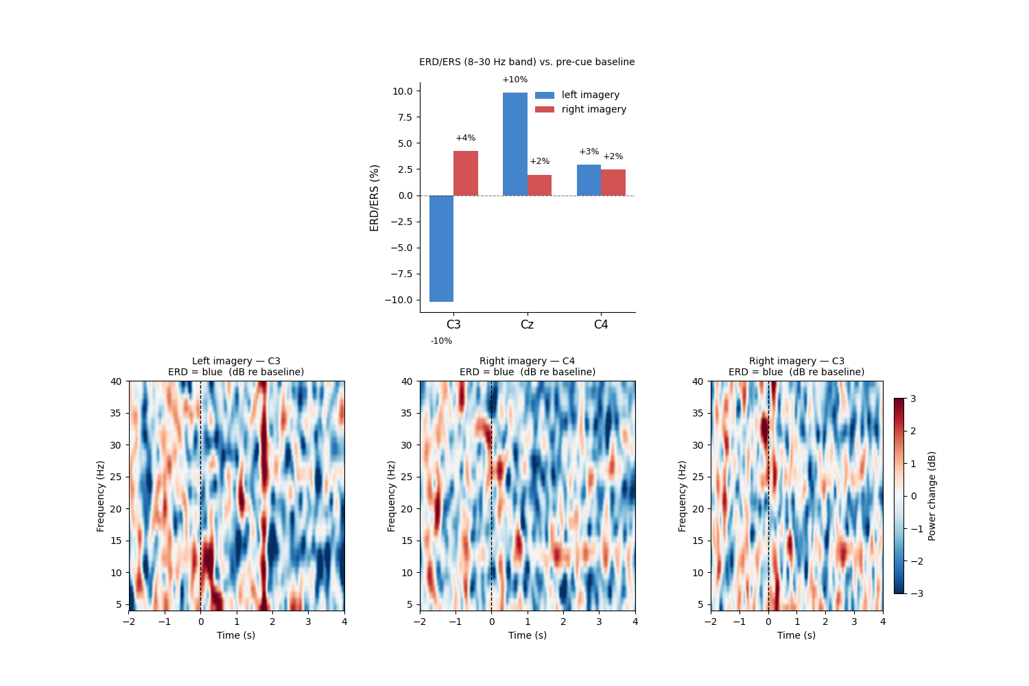
Compute ERD/ERS in the mu + beta band (8–30 Hz)

ERD/ERS is defined relative to a pre-cue baseline power:

\[\text{ERD/ERS}(\%) = \frac{P_{\text{active}} - P_{\text{baseline}}}{P_{\text{baseline}}} \times 100\]

Values < 0 = desynchronisation (ERD, power decrease during imagery). Values > 0 = synchronisation (ERS, rebound after imagery offset).

def _band_power(data, sfreq, fmin=8.0, fmax=30.0):
    sos = butter(4, [fmin, fmax], btype="bandpass", fs=sfreq, output="sos")
    filtered = sosfiltfilt(sos, data, axis=-1)
    return np.mean(filtered ** 2, axis=-1)


t_epoch   = epochs.times
base_mask = (t_epoch >= BASELINE[0]) & (t_epoch < BASELINE[1])
act_mask  = (t_epoch >= 0.5) & (t_epoch <= 3.5)
ch_idx    = {ch: i for i, ch in enumerate(["C3", "Cz", "C4"])}

erd_data = {}
for label in ("left", "right"):
    ep_data = epochs[label].get_data()
    base_pw = _band_power(ep_data[:, :, base_mask], SFREQ)
    act_pw  = _band_power(ep_data[:, :, act_mask],  SFREQ)
    erd_data[label] = (act_pw - base_pw) / (base_pw + 1e-30) * 100.0

for label in ("left", "right"):
    c3_erd = erd_data[label][:, ch_idx["C3"]].mean()
    c4_erd = erd_data[label][:, ch_idx["C4"]].mean()
    print(f"{label:5s} imagery — C3 ERD: {c3_erd:+.1f}%  C4 ERD: {c4_erd:+.1f}%")

left  imagery — C3 ERD: -10.2%  C4 ERD: +2.9%
right imagery — C3 ERD: +4.2%  C4 ERD: +2.5%

Time-frequency analysis

Morlet wavelet power is computed trial-by-trial and averaged. The 1.5 s pre-cue baseline (−2.0 to −0.5 s) is then used to express each time-frequency cell in decibels:

\[\text{TFR}_{\text{dB}}(f,t) = 10 \cdot \log_{10}\!\left(\frac{P(f,t)}{P_{\text{baseline}}(f)}\right)\]

Negative dB = ERD (power below baseline), positive dB = ERS.

freqs    = np.arange(4.0, 41.0, 1.0)
n_cycles = freqs / 2.0

tfr = {}
for label in ("left", "right"):
    tfr[label] = mne.time_frequency.tfr_array_morlet(
        epochs[label].get_data(),
        sfreq=SFREQ,
        freqs=freqs,
        n_cycles=n_cycles,
        output="power",
    ).mean(axis=0)

Real-time NF session with simulated motor lateralisation

Instead of streaming the mixed PhysioNet recording (rest + both imagery classes interleaved), we use simulate_raw() to synthesise a 64-channel biosemi64 EEG with a right-hemisphere mu (12 Hz) source in precentral-rh, alternating in 10 s ON / 10 s OFF bursts. During ON bursts C4 receives the strongest forward-model projection and laterality = (C4 − C3)/(C4 + C3) is clearly positive.

The ZScoreProtocol with direction="up" rewards windows where C4 dominates, mimicking a closed-loop right-hemisphere mu enhancement protocol (contralateral to left-hand imagery).

Expected mu-ON windows in the 120 s main session:

Main t (s): 0──2  12──22  32──42  52──62  72──82  92──102  112──120
            ■■■   ██████  ██████  ██████  ██████  ███████   ████

_tmp_dir = Path(tempfile.mkdtemp())
fname_motor = _tmp_dir / "motor_sim.fif"
simulate_raw(
    brain_label="precentral-rh",
    frequency=12.0,
    amplitude=50.0,
    duration=10.0,
    gap_duration=20.0,
    n_repetition=7,
    start=2.0,
    data_type="eeg",
    sfreq=256.0,
    fname_save=str(fname_motor),
    verbose=False,
)

protocol = ZScoreProtocol(
    direction="up",
    warmup_windows=20,
    zscore_threshold=0.5,
)

nf = RTStream(
    subject_id="motor01",
    session="01",
    subjects_dir=str(_tmp_dir),
    montage="biosemi64",
    data_type="eeg",
    verbose=False,
)
nf.connect_to_lsl(mock_lsl=True, fname=str(fname_motor), verbose=False)
nf.record_baseline(baseline_duration=10, verbose=False)
nf.record_main(
    duration=120,
    modality=["laterality"],
    winsize=2.0,
    signal_smoothing=0.3,
    protocol=protocol,
    show_nf_signal=False,
    show_raw_signal=False,
    show_topo=False,
    verbose=False,
)

lat_arr    = np.asarray(nf.nf_data.get("laterality", []))
reward_vals = np.asarray(nf.reward_data.get("laterality", []))
reward_arr  = reward_vals > 0

print(f"NF windows : {len(lat_arr)}  |  rewards : {int(reward_arr.sum())}  "
      f"({100*reward_arr.mean():.0f} % of all windows)")

/Users/payamsadeghishabestari/ANT/docs/source/../../src/mne_rt/tools/simulation.py:220: RuntimeWarning: No average EEG reference present in info["projs"], covariance may be adversely affected. Consider recomputing covariance using with an average eeg reference projector added.
  add_noise(raw, cov, iir_filter=iir_filter, verbose=verbose)
/Users/payamsadeghishabestari/ANT/docs/source/../../src/mne_rt/tools/simulation.py:231: RuntimeWarning: This filename (/var/folders/20/hsy69tx529ndn3rkv5gzcf0c0000gn/T/tmpxyteoxk9/motor_sim.fif) does not conform to MNE naming conventions. All raw files should end with raw.fif, raw_sss.fif, raw_tsss.fif, _meg.fif, _eeg.fif, _ieeg.fif, raw.fif.gz, raw_sss.fif.gz, raw_tsss.fif.gz, _meg.fif.gz, _eeg.fif.gz or _ieeg.fif.gz
  raw.save(fname=Path(fname_save), overwrite=True)
/Users/payamsadeghishabestari/ANT/docs/source/../../src/mne_rt/rt_stream.py:416: RuntimeWarning: This filename (/var/folders/20/hsy69tx529ndn3rkv5gzcf0c0000gn/T/tmpxyteoxk9/motor_sim.fif) does not conform to MNE naming conventions. All raw files should end with raw.fif, raw_sss.fif, raw_tsss.fif, _meg.fif, _eeg.fif, _ieeg.fif, raw.fif.gz, raw_sss.fif.gz, raw_tsss.fif.gz, _meg.fif.gz, _eeg.fif.gz or _ieeg.fif.gz
  self._mock_player = Player(
/Users/payamsadeghishabestari/ANT/docs/source/../../src/mne_rt/tools/tools.py:502: RuntimeWarning: No average EEG reference present in info["projs"], covariance may be adversely affected. Consider recomputing covariance using with an average eeg reference projector added.
  inverse_operator = make_inverse_operator(
/Users/payamsadeghishabestari/ANT/docs/source/../../src/mne_rt/tools/tools.py:502: RuntimeWarning: No average EEG reference present in info["projs"], covariance may be adversely affected. Consider recomputing covariance using with an average eeg reference projector added.
  inverse_operator = make_inverse_operator(
NF windows : 120  |  rewards : 53  (44 % of all windows)

Figure 1 — ERD/ERS bar chart and TFR

fig1, axes = plt.subplots(2, 3, figsize=(15, 10),
                           gridspec_kw={"hspace": 0.30, "wspace": 0.35})

ax_bar = axes[0, 1]
x      = np.arange(3)
w      = 0.33
colors = {"left": "#1565C0", "right": "#C62828"}

for i_label, (label, color) in enumerate(colors.items()):
    vals = [erd_data[label][:, ch_idx[ch]].mean() for ch in ["C3", "Cz", "C4"]]
    bars = ax_bar.bar(x + (i_label - 0.5) * w, vals, w,
                      color=color, alpha=0.80, label=f"{label} imagery")
    for bar, val in zip(bars, vals):
        ax_bar.text(bar.get_x() + bar.get_width() / 2,
                    bar.get_height() + (1 if val >= 0 else -4),
                    f"{val:+.0f}%", ha="center", fontsize=9)

ax_bar.axhline(0, color="black", lw=0.8, ls="--", alpha=0.5)
ax_bar.set_xticks(x)
ax_bar.set_xticklabels(["C3", "Cz", "C4"], fontsize=12)
ax_bar.set_ylabel("ERD/ERS (%)", fontsize=11)
ax_bar.set_title("ERD/ERS (8–30 Hz band) vs. pre-cue baseline\n", fontsize=10)
ax_bar.legend(fontsize=10, frameon=False)
ax_bar.spines[["top", "right"]].set_visible(False)
axes[0, 0].axis("off")
axes[0, 2].axis("off")

tfr_pairs = [("left", "C3"), ("right", "C4"), ("right", "C3")]

for ax, (label, ch) in zip(axes[1, :], tfr_pairs):
    ci        = ch_idx[ch]
    tf        = tfr[label][ci]
    base_cols = (t_epoch >= BASELINE[0]) & (t_epoch < BASELINE[1])
    base_mean = tf[:, base_cols].mean(axis=1, keepdims=True)
    tf_db     = 10.0 * np.log10(tf / (base_mean + 1e-30))

    im = ax.imshow(
        tf_db, aspect="auto", origin="lower",
        extent=[t_epoch[0], t_epoch[-1], freqs[0], freqs[-1]],
        cmap="RdBu_r", vmin=-3, vmax=3
    )
    ax.axvline(0, color="k", lw=1.0, ls="--")
    ax.set_xlabel("Time (s)", fontsize=10)
    ax.set_ylabel("Frequency (Hz)", fontsize=10)
    ax.set_title(f"{label.capitalize()} imagery — {ch}\nERD = blue  (dB re baseline)",
                 fontsize=10)
plt.colorbar(im, ax=ax, label="Power change (dB)", shrink=0.85)

fig1.tight_layout()

/Users/payamsadeghishabestari/ANT/examples/ex_motor_imagery_nf.py:278: UserWarning: This figure includes Axes that are not compatible with tight_layout, so results might be incorrect.
  fig1.tight_layout()

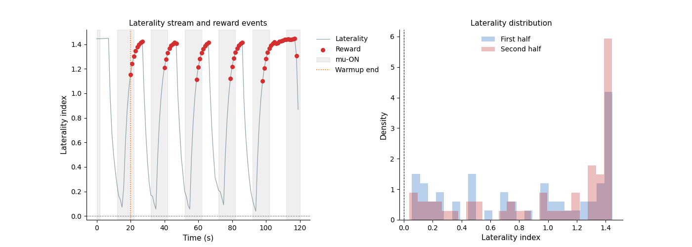
Figure 2 — Real-time NF stream

Laterality index and reward delivery events from the simulated ANT session. Grey bands mark expected mu-ON periods; rewards should align with them.

# mu-ON windows (seconds, relative to main-session start)
_mu_on = [(0, 2), (12, 22), (32, 42), (52, 62), (72, 82), (92, 102), (112, 120)]
hop_s  = 1.0   # winsize=2.0 s with 50 % overlap → 1 s per step

fig2, (ax_lat, ax_hist) = plt.subplots(1, 2, figsize=(14, 5),
                                        gridspec_kw={"wspace": 0.40})

t_s = np.arange(len(lat_arr)) * hop_s
ax_lat.plot(t_s, lat_arr, color="#607D8B", lw=0.9, alpha=0.7, label="Laterality")
ax_lat.scatter(t_s[reward_arr], lat_arr[reward_arr],
               s=30, color="#D32F2F", zorder=5, label="Reward")
for t0, t1 in _mu_on:
    ax_lat.axvspan(t0, t1, alpha=0.12, color="grey",
                   label="mu-ON" if t0 == 0 else None)
ax_lat.axhline(0, color="k", lw=0.7, ls="--", alpha=0.5)
ax_lat.axvline(20, color="#FF6F00", lw=1.2, ls=":", label="Warmup end")
ax_lat.set_xlabel("Time (s)", fontsize=11)
ax_lat.set_ylabel("Laterality index", fontsize=11)
ax_lat.set_title("Laterality stream and reward events", fontsize=11)
ax_lat.legend(fontsize=10, frameon=False, bbox_to_anchor=(1, 1))
ax_lat.spines[["top", "right"]].set_visible(False)

half = len(lat_arr) // 2
ax_hist.hist(lat_arr[:half], bins=25, alpha=0.3, color="#1565C0",
             density=True, label="First half")
ax_hist.hist(lat_arr[half:], bins=25, alpha=0.3, color="#C62828",
             density=True, label="Second half")
ax_hist.axvline(0, color="k", lw=0.8, ls="--")
ax_hist.set_xlabel("Laterality index", fontsize=11)
ax_hist.set_ylabel("Density", fontsize=11)
ax_hist.set_title("Laterality distribution", fontsize=11)
ax_hist.legend(fontsize=10, frameon=False)
ax_hist.spines[["top", "right"]].set_visible(False)

fig2.tight_layout()

/Users/payamsadeghishabestari/ANT/examples/ex_motor_imagery_nf.py:320: UserWarning: This figure includes Axes that are not compatible with tight_layout, so results might be incorrect.
  fig2.tight_layout()