Compare different neurofeedback method delays

This example shows how to visualize delays for different neurofeedback methods using Seaborn’s FacetGrid and KDE plots.

Now let’s load data and visualize each method’s delay.

from pathlib import Path
import pandas as pd
import matplotlib.pyplot as plt
import seaborn as sns

fname = Path.cwd().parent / "data" / "sample" / "method_delays.csv"
df = pd.read_csv(fname, index_col=0)

Helper function for labeling each row

def label(x, color, label):
    ax = plt.gca()
    ax.text(0.8, .2, label, fontweight="bold", fontstyle='italic', color=color,
            ha="left", va="center", transform=ax.transAxes)

Function to plot KDEs for a list of methods

def plot_method_delays(df, method_names, xlim, ylim, bw_adjust=1, top=0.72):
    """
    Plot KDEs of delays for specified neurofeedback methods.

    Parameters
    ----------
    df : pandas.DataFrame
        Must contain columns 'method' and 'delay'.
    method_names : list of str
        Methods to plot.
    xlim : list of float
        X-axis limits.
    ylim : list of float
        Y-axis limits.
    bw_adjust : float, optional
        Bandwidth adjustment for KDE (default 1).
    top : float, optional
        Top position for FacetGrid (default 0.72).

    Returns
    -------
    g : seaborn.FacetGrid
        FacetGrid object.
    """
    df_sub = df.query("method == @method_names")
    pal = sns.cubehelix_palette(len(method_names), rot=-.2, light=.7)

    g = sns.FacetGrid(
        df_sub, row="method", hue="method", aspect=14, height=.75,
        palette=pal, row_order=method_names, xlim=xlim, ylim=ylim
    )

    g.map(sns.kdeplot, "delay", bw_adjust=bw_adjust, clip_on=False, clip=xlim,
            fill=True, alpha=1, linewidth=1.5)
    g.map(sns.kdeplot, "delay", clip_on=False, color="w", clip=xlim,
            lw=2, bw_adjust=bw_adjust)
    g.refline(y=0, linewidth=2, linestyle="-", color=None, clip_on=False)
    g.map(label, "delay")

    g.figure.subplots_adjust(hspace=.15, top=top)
    g.set_titles("")
    g.set(yticks=[], ylabel="", xlabel=r"method delay ($m s$)")
    g.despine(bottom=True, left=True)
    return g

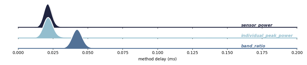
Now let’s visualize delays for “sensor_power”, “individual_peak_power”, “band_ratio”

plot_method_delays(
    df,
    ["sensor_power", "individual_peak_power", "band_ratio"],
    xlim=[0, 0.2],
    ylim=[0, 50]
)
plt.show()

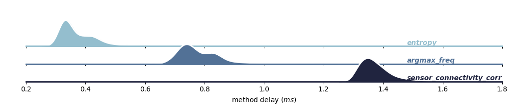
Next, visualize delays for “entropy”, “argmax_freq”, “sensor_connectivity_corr”

plot_method_delays(
    df,
    ["entropy", "argmax_freq", "sensor_connectivity_corr"],
    xlim=[0.2, 1.8],
    ylim=[0, 6],
    bw_adjust=1.5
)
plt.show()

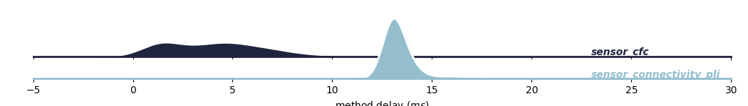
Next, visualize delays for “sensor_cfc”, “sensor_connectivity_pli”

plot_method_delays(
    df,
    ["sensor_cfc", "sensor_connectivity_pli"],
    xlim=[-5, 30],
    ylim=[0, 0.2],
    bw_adjust=1.8,
    top=0.65
)
plt.show()

/Users/payamsadeghishabestari/ANT/venv/lib/python3.10/site-packages/seaborn/axisgrid.py:123: UserWarning: Tight layout not applied. tight_layout cannot make Axes height small enough to accommodate all Axes decorations.
  self._figure.tight_layout(*args, **kwargs)
/Users/payamsadeghishabestari/ANT/venv/lib/python3.10/site-packages/seaborn/axisgrid.py:123: UserWarning: Tight layout not applied. tight_layout cannot make Axes height small enough to accommodate all Axes decorations.
  self._figure.tight_layout(*args, **kwargs)
/Users/payamsadeghishabestari/ANT/venv/lib/python3.10/site-packages/seaborn/axisgrid.py:123: UserWarning: Tight layout not applied. tight_layout cannot make Axes height small enough to accommodate all Axes decorations.
  self._figure.tight_layout(*args, **kwargs)
/Users/payamsadeghishabestari/ANT/venv/lib/python3.10/site-packages/seaborn/axisgrid.py:123: UserWarning: Tight layout not applied. tight_layout cannot make Axes height small enough to accommodate all Axes decorations.
  self._figure.tight_layout(*args, **kwargs)

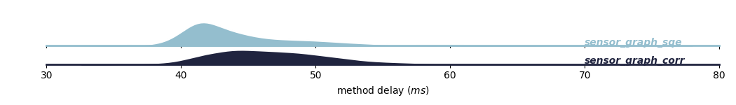
Next, visualize delays for “sensor_graph_sqe”, “sensor_graph_corr”

plot_method_delays(
    df,
    ["sensor_graph_sqe", "sensor_graph_corr"],
    xlim=[30, 80],
    ylim=[0, 0.1]
)
plt.show()

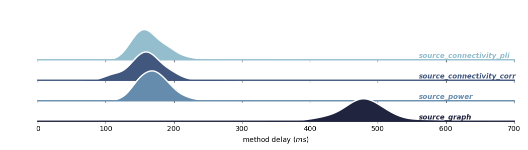
Finally, visualize delays for “source_connectivity_pli”, “source_connectivity_corr”, “source_power”, “source_graph”

plot_method_delays(
    df,
    ["source_connectivity_pli", "source_connectivity_corr",
     "source_power", "source_graph"],
    xlim=[0, 700],
    ylim=[0, 0.01],
    bw_adjust=1.5
)
plt.show()